Regularization and Generalized Linear Models

In this section, we will leverage the context of linear models established earlier to discuss the problem of overfitting and regularization methods for addressing it. Regularization is a general technique applicable to many models including linear models and neural networks, but because the parameters of linear models directly correspond to feature influence, regularization prevents overfitting while maintaining model interpretability by constraining parameter magnitude, and it has a perfect geometric interpretation (the intersection of contour lines and constraint regions). In contrast, the parameters of neural network models are distributed representations, making the effect of regularization relatively abstract and difficult to understand intuitively.

Computer scientist Arthur Samuel, while developing a machine learning checkers program, discovered that the program performed well on the training set but frequently made mistakes in actual gameplay. The reason was that the model had over-learned the details of the training data, losing its grasp of the true underlying patterns. It is like a high school student who chooses to memorize past college entrance exam questions rather than truly understanding the knowledge — naturally, they struggle to achieve good scores on the actual exam. Samuel named this phenomenon Overfitting, and Regularization is the key technique used to solve overfitting. It works by adding parameter constraints to the loss function, forcing the model to break free from the complex details of the training data and seek simpler structures to fit the data.

Fitting and Generalization

The goal of machine learning is never to "memorize the training data," but rather to "learn to predict the unknown." Generalization refers to the model's ability to transfer knowledge learned from the training set to the test set. The training set is the "textbook," the test set is the "exam," and whether you've learned well is only determined by the exam. The mathematical definition of generalization is the model's expected error over the entire data distribution:

$$E_{generalization} = \mathbb{E}_{(x,y) \sim P_{true}}[L(f(x), y)]$$

However, in practice, we cannot access all the data from the "true distribution" and can only learn from a limited training set and evaluate on a limited test set. Therefore, generalization ability is typically measured by the gap between test error and training error:

• Large training error, large test error: This phenomenon is called Underfitting, indicating that the model itself has not been trained sufficiently. Training itself is a gradual process from underfitting to fitting, and continuing iterative optimization is the remedy.
• Small training error, small test error: This phenomenon indicates that the model generalizes well and has learned the true patterns — this is the result we want.
• Small training error, large test error: This phenomenon is called Overfitting, indicating poor generalization ability. It requires adjusting the model structure, changing the training method, and other measures to address.

Consider a concrete example of how to choose different models to fit real-world data. Suppose the task is to learn a fitting curve from 10 data points, where the true data generation process is $y = \sin(x) + \text{noise}$. You have the following three models of varying complexity to choose from:

Model	Parameters	Training Error	Prediction on New Data
Linear model: $y = ax + b$	2	Large	Stable, poor generalization
Cubic polynomial: $y = a_0 + a_1x + a_2x^2 + a_3x^3$	4	Moderate	Relatively stable, good generalization
9th-degree polynomial: $y = \sum_{i=0}^{9} a_i x^i$	10	Near 0	Prediction fails, poor generalization

Since the 9th-degree polynomial has 10 parameters, exactly equal to the number of samples, the function curve can theoretically pass perfectly through every data point in the training set (training error near 0). However, this "perfect curve" will almost certainly make incorrect predictions on new data. With only 10 data points, it is fundamentally insufficient to support training a model of this complexity, and overfitting is almost inevitable. Overfitting arises from a combination of three factors:

1. Excessive model complexity: Too many parameters give the model enough degrees of freedom to fit noise rather than true patterns. In the example, the 9th-degree polynomial draws a curve through the scatter plot, allowing arbitrary bends (many parameters). It can pass through every noisy point, creating a jagged curve that is perfect on training data but worthless on new data.

2. Insufficient training data: Too few samples prevent the model from learning true statistical patterns. According to general statistical experience, the number of parameters should be significantly less than the number of samples (e.g., the sample size should be at least 10 times the number of parameters); otherwise, the model is prone to overfitting.

3. Noise in training data: Noise in the training data is learned by the model as if it were a pattern. Real data always contains measurement errors, recording biases, and other noise. When model complexity is sufficiently high, it will diligently learn this noise, leading to inaccurate predictions.

Regularization Principle

Among the three sources of overfitting listed above, the third — noise — is a limitation of the data source itself and cannot be controlled manually, only mitigated as much as possible through data preprocessing, so we will not discuss it here. The first two essentially boil down to the same statement: the training data is insufficient to support the model's complexity. Previously, our only optimization goal was to minimize the loss function. If in engineering practice we set the sole training objective as minimizing the loss function, we can easily obtain a highly intricate but extremely fragile model that outperforms a robust, simple model on the training set — which is clearly not the result we want. Therefore, we need to establish a second objective for model optimization besides minimizing the loss function: limiting model complexity. The principle of regularization is to add a parameter penalty term to the loss function to constrain model complexity, expressed mathematically as:

$$L_{reg}(\beta) = L(\beta) + \lambda \cdot R(\beta)$$

where $L(\beta)$ is the original loss function (e.g., squared loss for linear regression, cross-entropy loss for logistic regression), $R(\beta)$ is the regularization term that penalizes the number and magnitude of parameters, and $\lambda$ is the regularization strength that controls the penalty intensity.

The 9th-degree polynomial example already illustrates the impact of the number of parameters on model complexity. Additionally, excessively large parameter values also pose an overfitting risk. Large parameter values mean the model is overly sensitive to input features, where tiny changes in input lead to enormous changes in output. Imagine a linear regression model $y = 1000x_1 + 0.01x_2$: when $x_1$ changes by 1, the output changes by 1000; when $x_2$ changes by 100, the output changes by only 1. This extreme sensitivity disparity is a hallmark of overfitting — the model overreacts to certain features, likely treating noise as a genuine pattern.

L1 Regularization: Lasso

Lasso (Least Absolute Shrinkage and Selection Operator) is also commonly referred to directly as L1 regularization. It is mainly used to constrain the number of model parameters and can drive some parameters to exactly zero. A parameter of zero means the corresponding feature is eliminated, and the model learns only the truly useful features. This automatic feature selection capability is called sparsity, which is the core value that distinguishes L1 regularization from other forms. The mathematical expression of Lasso is: $L_{Lasso}(\beta) = L(\beta) + \lambda ||\beta||_1$, where $||\beta||_1 = \sum_{j=1}^{d} |\beta_j|$ is the sum of absolute parameter values, i.e., the L1 norm of the parameters. To clearly explain how L1 regularization achieves sparsity, let us first revisit the shape of the L1 unit ball in norms, as shown in the figure below:

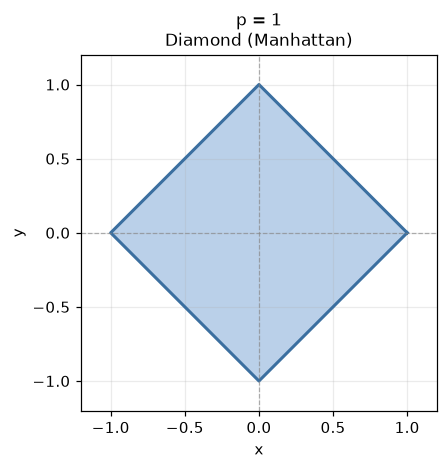
L1 unit ball image

The absolute value function $|\beta|$ has a "cusp" at $\beta = 0$: the left derivative is -1, the right derivative is +1, they are not equal, and the function is non-differentiable at this point. This non-differentiable point acts like a trap — when a parameter is optimized to near zero, the gradient direction suddenly changes, and the parameter tends to get stuck at zero, unable to move further. To use an analogy: imagine you are walking downhill. The hill of L1 regularization has a "V-shaped depression" at $\beta = 0$. When you reach the bottom of the depression, the slopes on both sides go upward, so you naturally stop there. The hill of L2 regularization, which we will introduce shortly, is smooth and bowl-shaped, without such a depression — you will only slide to a position near zero, but not exactly zero.

Consider a concrete example. Suppose the model has only two parameters $\beta_1$ and $\beta_2$. We still set the optimization goal as minimizing the loss function, but add a constraint $|\beta_1| + |\beta_2| \leq 1$. This constraint forms a diamond-shaped region on the plane, with four "corners" located at $(1, 0)$, $(0, 1)$, $(-1, 0)$, and $(0, -1)$, which happen to lie on the coordinate axes.

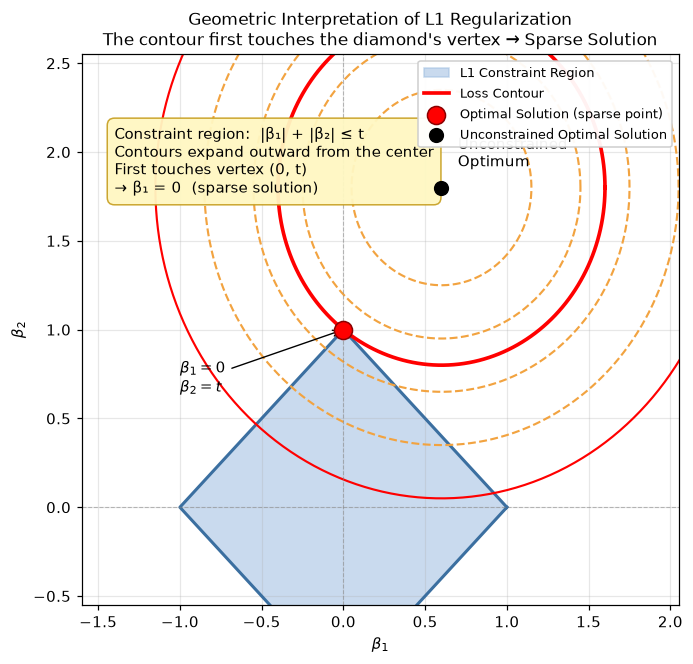
Geometric explanation of L1 regularization producing sparse solutions: the loss function contour (red ellipse) first touches a corner of the diamond, yielding a sparse solution

During iterative optimization, without constraints, the optimal solution of the loss function can be anywhere. With the constraint, the loss function cannot reach its minimum and must progressively seek the next smallest value until the constraint is satisfied. Drawing contours for these progressively approximated suboptimal values (imagine the loss function image previously likened to peaks/valleys — contours are like the topographical lines of those peaks/valleys), we can see that the contours expand outward from the center point representing the minimum. The first point of contact between a contour and the constraint region is the optimal solution under the constraint. Since the diamond's boundary consists of straight lines, the contour is more likely to hit the diamond's corners (sharp angles) rather than the flat edges. Hitting a corner means one parameter is zero — this is the geometric origin of sparse solutions.

Sparse solutions are equivalent to automatic feature selection: features with zero coefficients are eliminated. Lasso automatically selects the most important features without manual filtering. This is extremely valuable in scenarios such as gene selection (identifying disease-causing genes from thousands of genes), text classification (selecting keywords from a vast vocabulary), and many others. Moreover, a simpler model enhances interpretability: a sparse solution retains only a small number of non-zero parameters, helping, for example, a doctor narrow down hundreds of complex lab results to a few key indicators, allowing the doctor to focus on explaining the cause.

Since Lasso has no closed-form solution (because $|\beta|$ is non-differentiable), it also requires iterative optimization algorithms. Coordinate descent is a common algorithm for Lasso regression. The general idea is to update only one parameter at a time while keeping the others fixed, cycling through them until convergence. The following code implements Lasso regression using the coordinate descent algorithm.

import numpy as np

class LassoRegression:
    """
    Lasso Regression Implementation (L1 Regularization)
    Uses Coordinate Descent Algorithm
    
    Suitable for:
    1. Automatic feature selection
    2. Large number of features, some may be irrelevant
    3. Pursuing sparse, interpretable models
    """
    
    def __init__(self, alpha=1.0, n_iterations=1000, tol=1e-4):
        self.alpha = alpha          # Regularization strength lambda
        self.n_iterations = n_iterations  # Maximum iterations
        self.tol = tol              # Convergence threshold
        self.coef_ = None
        self.intercept_ = None
    
    def soft_threshold(self, rho, lambda_):
        """
        Soft threshold function (core operation of Lasso)
        
        Pushes parameters toward zero, possibly reaching exactly zero
        """
        if rho < -lambda_:
            return rho + lambda_
        elif rho > lambda_:
            return rho - lambda_
        else:
            return 0.0
    
    def fit(self, X, y):
        """
        Train the model (coordinate descent)
        
        Updates one parameter at a time, cycling until convergence
        """
        n_samples, n_features = X.shape
        
        # Initialize parameters
        self.coef_ = np.zeros(n_features)
        self.intercept_ = np.mean(y)
        y_centered = y - self.intercept_
        
        # Standardize data (accelerate convergence, ensure fair penalization)
        X_mean = np.mean(X, axis=0)
        X_std = np.std(X, axis=0)
        X_std[X_std == 0] = 1  # Avoid division by zero
        X_normalized = (X - X_mean) / X_std
        
        # Coordinate descent iteration
        for iteration in range(self.n_iterations):
            coef_old = self.coef_.copy()
            
            for j in range(n_features):
                # Compute the "partial residual" for the current feature
                # i.e., the prediction residual after removing the j-th feature
                residual = y_centered - X_normalized @ self.coef_ + self.coef_[j] * X_normalized[:, j]
                
                # Compute rho (the unregularized gradient term)
                rho = X_normalized[:, j] @ residual / n_samples
                
                # Apply soft threshold (key step of Lasso)
                self.coef_[j] = self.soft_threshold(rho, self.alpha)
            
            # Check convergence (compare in standardized space)
            if np.max(np.abs(self.coef_ - coef_old)) < self.tol:
                break
        
        # Transform back to original scale (executed once after iteration)
        self.coef_ = self.coef_ / X_std
        self.intercept_ = self.intercept_ - X_mean @ self.coef_
        
        return self
    
    def predict(self, X):
        """Predict"""
        return X @ self.coef_ + self.intercept_
    
    def score(self, X, y):
        """R-squared score"""
        y_pred = self.predict(X)
        ss_res = np.sum((y - y_pred) ** 2)
        ss_tot = np.sum((y - np.mean(y)) ** 2)
        return 1 - ss_res / ss_tot
    
    def get_selected_features(self, threshold=0.01):
        """Return indices of selected features (non-zero coefficients)"""
        return np.where(np.abs(self.coef_) > threshold)[0]


# Demonstrate Lasso sparsity
n_samples = 100
n_features = 10

# Generate data: only 3 features are truly useful, the remaining 7 are noise
X = np.random.randn(n_samples, n_features)
true_coef = np.array([5, 3, -2, 0, 0, 0, 0, 0, 0, 0])  # Only first 3 are effective
y = X @ true_coef + np.random.randn(n_samples) * 0.5

# Lasso regression
lasso = LassoRegression(alpha=0.5, n_iterations=1000)
lasso.fit(X, y)

print("=== Lasso Sparsity Demonstration ===")
print(f"True coefficients: {true_coef}")
print(f"Lasso estimates: {lasso.coef_}")
print(f"R-squared score: {lasso.score(X, y):.3f}")
print(f"Number of non-zero parameters: {len(lasso.get_selected_features())} (originally {len(true_coef)})")
print("Lasso successfully identified the 3 truly useful features!")

Click Run to execute code. Click the code area to edit.

L2 Regularization: Ridge Regression

Ridge Regression is also commonly referred to directly as L2 regularization. Its main role is to constrain the magnitude of parameter values, making parameter estimates more stable, but it typically does not drive parameters to exactly zero. Parameter shrinkage means the model's response to all features becomes more moderate, reducing over-reliance on any single feature. This stability improvement is the core value that distinguishes Ridge regression from Lasso. The mathematical expression of Ridge regression is: $L_{Ridge}(\beta) = L(\beta) + \lambda ||\beta||^2_2$, where $||\beta||^2_2 = \sum_{j=1}^{d} \beta_j^2$ is the square of the L2 norm of the parameters.

Consider the same example used for Lasso: suppose the model has only two parameters $\beta_1$ and $\beta_2$, with the optimization goal still being loss function minimization, but the constraint becomes $\beta_1^2 + \beta_2^2 \leq 1$. This constraint forms a circular region on the plane, whose boundary is smooth and rounded everywhere, with no "corners" or "sharp points." When the contour lines of the loss function expand outward from the center, the point where they first touch the circular boundary typically does not fall on the coordinate axes — both parameters are non-zero. This is why L2 regularization does not produce sparse solutions.

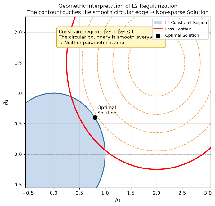
Geometric explanation of L2 regularization: the circular boundary is smooth, and when the contour touches the circle, neither parameter is zero

Non-sparsity means Ridge regression retains all features, only reducing their coefficients. When all features are genuinely useful (e.g., in house price prediction where area, number of rooms, and location score are all relevant), Ridge regression is a better choice than Lasso. Lasso may eliminate some relevant features due to sample data limitations, whereas Ridge regression preserves all information and stably handles collinearity (where multiple features are highly correlated, making it difficult for the model to distinguish the independent contribution of each feature, e.g., $x_2 \approx 2x_1$). The greatest advantage of Ridge regression is undoubtedly that it has a closed-form solution, requiring no iterative optimization — the optimal solution can be computed in a single pass with extremely high computational efficiency. The closed-form solution of Ridge regression is $\hat{\beta}_{Ridge} = (X^TX + \lambda I)^{-1}X^Ty$. Compared with the OLS closed-form solution $\hat{\beta}_{OLS} = (X^TX)^{-1}X^Ty$, Ridge regression adds $\lambda I$ to $X^TX$. This seemingly simple modification addresses three inherent shortcomings of OLS:

1. Always solvable: When collinearity exists among features, $X^TX$ may be non-invertible or nearly non-invertible (as discussed in matrix inversion, one of the three conditions for invertibility is full rank, and collinearity implies rank deficiency). OLS has no solution or produces extremely unstable parameter estimates. Ridge regression, by adding $\lambda I$, guarantees the matrix is always invertible — it is like laying a layer of gravel on a muddy road, making a previously impassable path usable.

2. Stable parameter shrinkage: The regularization term $\lambda\|\beta\|_2^2$ makes the parameter estimates smaller than those of OLS, pulling parameters toward the origin. This shrinkage effect reduces the model's dependence on individual features and improves generalization stability.

3. Reasonable handling of collinearity: When multiple features are highly correlated (e.g., "area" and "number of rooms" in house price prediction), OLS parameter estimates may fluctuate wildly (one feature coefficient is positive, another is negative, both with large absolute values). Ridge regression, through parameter constraints, makes the coefficients of correlated features tend to be similar, avoiding such unreasonable fluctuations.

The following table summarizes the characteristics and applicable scenarios of Ridge regression and Lasso:

Property	Ridge (L2)	Lasso (L1)
Parameter constraint	Shrinks but not to zero	Can be exactly zero (sparse)
Feature selection	Not automatic	Automatic
Computational complexity	Closed-form, fast	Requires iterative optimization
Collinearity handling	Parameters tend to be similar, stable	Randomly selects one to set to zero, unstable
Suitable scenarios	All features are relevant	Feature selection needed

The following code implements a complete Ridge regression class and demonstrates how Ridge regression handles collinearity. When features are highly correlated, Ridge regression constrains the parameter space through L2 regularization to obtain a stable solution, making the coefficients of correlated features tend to be similar, rather than randomly zeroing one out as Lasso does.

import numpy as np

class RidgeRegression:
    """
    Ridge Regression Implementation (L2 Regularization)
    
    Suitable for:
    1. Collinearity among features
    2. Unstable parameter estimates
    3. Preventing overfitting
    """
    
    def __init__(self, alpha=1.0):
        self.alpha = alpha  # Regularization strength lambda
        self.coef_ = None   # Feature coefficients
        self.intercept_ = None  # Intercept
    
    def fit(self, X, y):
        """
        Train the model (closed-form solution)
        
        Parameters:
        X : ndarray, shape (n_samples, n_features)
            Feature matrix
        y : ndarray, shape (n_samples,)
            Target vector
        """
        n_samples = X.shape[0]
        X_augmented = np.column_stack([np.ones(n_samples), X])
        
        # Ridge regression closed-form solution: beta = (X^T X + lambda*I)^(-1) X^T y
        # Note: intercept is not regularized (first element of I is set to 0)
        I = np.eye(X_augmented.shape[1])
        I[0, 0] = 0  # Intercept term excluded from regularization
        
        XtX = X_augmented.T @ X_augmented
        Xty = X_augmented.T @ y
        
        self.beta_ = np.linalg.solve(XtX + self.alpha * I, Xty)
        
        self.intercept_ = self.beta_[0]
        self.coef_ = self.beta_[1:]
        
        return self
    
    def predict(self, X):
        """Predict"""
        return X @ self.coef_ + self.intercept_
    
    def score(self, X, y):
        """R-squared score"""
        y_pred = self.predict(X)
        ss_res = np.sum((y - y_pred) ** 2)
        ss_tot = np.sum((y - np.mean(y)) ** 2)
        return 1 - ss_res / ss_tot


# Demonstration: collinearity problem
n_samples = 50

# Generate highly correlated features (simulate collinearity)
x1 = np.random.randn(n_samples)
x2 = x1 + np.random.randn(n_samples) * 0.01  # x2 is almost equal to x1 (high collinearity)
x3 = np.random.randn(n_samples)
X = np.column_stack([x1, x2, x3])

# Target: true pattern is that x1 and x3 have influence, x2 should be unimportant (but x2 ≈ x1)
y = 2 * x1 + 3 * x3 + np.random.randn(n_samples) * 0.5

print("=== Collinearity Demonstration ===")
print("Feature correlation: x1 and x2 are highly correlated (≈0.99)")

# OLS attempt (may be numerically unstable)
try:
    X_aug = np.column_stack([np.ones(n_samples), X])
    XtX = X_aug.T @ X_aug
    beta_ols = np.linalg.solve(XtX, X_aug.T @ y)
    print(f"OLS parameters: {beta_ols[1:]}")
    print("Warning: OLS parameters may be unstable due to collinearity!")
except np.linalg.LinAlgError:
    print("OLS failed: matrix is singular!")

# Ridge regression (stable handling of collinearity)
ridge = RidgeRegression(alpha=1.0)
ridge.fit(X, y)
print(f"Ridge parameters: {ridge.coef_}")
print(f"Ridge R-squared: {ridge.score(X, y):.3f}")
print("Ridge parameters are more stable, coefficients of correlated features tend to be similar")

Click Run to execute code. Click the code area to edit.

Generalized Linear Model

We have already studied linear regression and logistic regression. They have different applicable tasks (regression vs. classification), different loss functions (squared error vs. cross-entropy), and different optimization methods (OLS closed-form vs. iterative optimization), yet they seem to share the same underlying framework for problem-solving (finding hypotheses, establishing criteria, measuring loss, optimizing the model). Using a real-life analogy: it is like learning two instruments — piano and violin. On the surface, the piano uses a keyboard, the violin uses strings, and the playing postures are completely different. But as you study deeper, you realize they share the same musical theory foundation: scales, rhythm, chords, and so on. The Generalized Linear Model (GLM) framework is like the theory that reveals this unity in music — it tells us that linear regression and logistic regression are different on the surface, but their "playing techniques" (mathematical essence) are connected. The similarity between the two begins to emerge from this comparison table:

Aspect	Linear Regression	Logistic Regression
Task type	Regression (predicting values)	Classification (predicting categories)
Loss function	Squared loss	Cross-entropy loss
Parameter estimation	OLS closed-form	Gradient descent iteration
Output range	$(-\infty, +\infty)$	$(0, 1)$
Linear predictor	$X\beta$	$X\beta$
Distribution assumption	Normal distribution	Bernoulli distribution

The differences in the first four rows of the table are obvious, but note the last two rows: both have the same linear predictor $X\beta$, differing only in output method and distribution assumption. This is like the piano and violin — though they are played differently, both perform the same musical score (the linear predictor). The GLM framework is precisely intended to reveal this score consistency. It uses three elements to define the relationship between the response variable $y$ and the linear predictor $X\beta$, mathematically expressed as $\mathbb{E}[y] = g^{-1}(X\beta)$. Here $g$ is called the link function, responsible for transforming the output of the linear predictor $X\beta$ into the range of the response variable. The combination of these three elements in this formula can generate a rich family of GLM models:

1. Distribution family: The distribution that the response variable $y$ follows is the model's assumption about the data generation mechanism. Linear regression assumes $y$ follows a normal distribution (continuous values), logistic regression assumes $y$ follows a Bernoulli distribution (binary classification), Poisson regression assumes $y$ follows a Poisson distribution (count values), and so on.

2. Linear predictor: $X\beta$ is the common computational engine for all GLMs, linearly combining input features to compute a score for each sample. Regardless of the subsequent transformation, the first step is always computing $X\beta$.

3. Link function: $g$ connects the linear predictor to the distribution mean $\mu$. Its role is to translate the raw output of $X\beta$ to an appropriate value range. Linear regression needs no translation, so $g(\mu) = \mu$ (Identity link). Logistic regression needs to map $X\beta$ to probability $(0, 1)$, so it uses the Logit link function.

The most valuable aspect of the GLM framework is that it brings seemingly different models under a unified perspective. The following table shows four common GLMs:

Model	Distribution Family	Link Function	Link Function Formula	Typical Application
Linear regression	Normal	Identity	$g(\mu) = \mu$	House price prediction
Logistic regression	Bernoulli	Logit	$g(\mu) = \log\frac{\mu}{1-\mu}$	Customer churn diagnosis
Poisson regression	Poisson	Log	$g(\mu) = \log\mu$	Traffic flow prediction
Probit regression	Bernoulli	Probit	$g(\mu) = \Phi^{-1}(\mu)$	Credit scoring

Let us take logistic regression as an example and re-examine its operating mechanism through the lens of the GLM framework:

• Distribution family: The label $y$ follows a Bernoulli distribution, with probability $p$ for $y=1$ and $1-p$ for $y=0$. This corresponds to the fact that the outcome of a classification task can only be one of two categories.

• Linear predictor: $z = X\beta$ computes a score for each sample. The score $z$ can be any real number (e.g., -5.3 or 8.7), but we need a probability $p \in (0, 1)$.

• Link function: The Logit function $g(p) = \log\frac{p}{1-p}$ (log-odds) builds a bridge between the score $z$ and the probability $p$. The formula $z = g(p) = \log\frac{p}{1-p}$ can be inverted to $p = \frac{1}{1+e^{-z}} = \sigma(z)$, which is the Sigmoid transformation.

The GLM framework reveals the standard operating procedure of logistic regression: first compute the linear predictor $X\beta$, then use the Sigmoid function to map it to the probability range. Linear regression is more direct: $X\beta$ itself is the predicted value, requiring no additional transformation. Understanding the GLM framework is like learning music theory and then picking up a new instrument — you know the new instrument is just a different mode of expression, and the underlying principles are the same.

Regularization in Practice

The following code uses a simulated house price prediction scenario to intuitively demonstrate the differences between L1 and L2 regularization. We generate 20 candidate features, but only the first 5 features truly affect house prices (with coefficients 50, 30, -20, 15, 10 respectively), and the remaining 15 are irrelevant noise features. By comparing Ridge regression (lambda=1) and two Lasso variants with different strengths (lambda=0.5, lambda=2), we can observe:

• Coefficient shrinkage: Ridge regression shrinks all feature coefficients toward zero but not to zero; Lasso compresses some coefficients to exactly zero.
• Feature selection effect: Lasso with strong regularization (lambda=2) has a high probability (depending on random data) of successfully eliminating all noise features, retaining only the 5 effective features.
• Prediction performance balance: The regularization strength requires a trade-off between fitting ability and sparsity — too weak leaves noise, too strong loses information.

import numpy as np
import matplotlib.pyplot as plt
from shared.linear.ridge_regression import RidgeRegression
from shared.linear.lasso_regression import LassoRegression

# Simulate house price prediction data
n_samples = 100
n_features = 20  # 20 candidate features, but only 5 are truly useful

# Generate features
X = np.random.randn(n_samples, n_features)

# True pattern: only the first 5 features affect house prices
true_coef = np.array([50, 30, -20, 15, 10, 0, 0, 0, 0, 0, 0, 0, 0, 0, 0, 0, 0, 0, 0, 0])
y = X @ true_coef + np.random.randn(n_samples) * 10

# Train three models
models = {
    'Ridge (lambda=1)': RidgeRegression(alpha=1.0),
    'Lasso (lambda=0.5)': LassoRegression(alpha=0.5),
    'Lasso (lambda=2)': LassoRegression(alpha=2.0)
}

results = {}
for name, model in models.items():
    model.fit(X, y)
    results[name] = {
        'coef': model.coef_,
        'score': model.score(X, y),
        'nonzero': np.sum(np.abs(model.coef_) > 0.01)
    }

# Visualization comparison
fig, axes = plt.subplots(1, 3, figsize=(15, 5))

# Figure 1: Coefficient comparison
colors = {'Ridge (lambda=1)': '#3498db', 'Lasso (lambda=0.5)': '#e74c3c', 'Lasso (lambda=2)': '#9b59b6'}
for i, (name, res) in enumerate(results.items()):
    axes[0].bar(np.arange(n_features) + i*0.25, res['coef'], width=0.25, 
                color=colors[name], alpha=0.7, label=name)

axes[0].axhline(y=0, color='black', linewidth=0.5)
axes[0].set_xlabel('Feature index')
axes[0].set_ylabel('Coefficient value')
axes[0].set_title('Coefficient comparison of different regularization methods')
axes[0].legend()

# Mark truly effective features
axes[0].axvspan(-0.5, 4.5, alpha=0.1, color='green', label='Truly effective features')

# Figure 2: Model performance vs. feature count (dual-axis chart)
model_names = list(results.keys())
scores = [results[n]['score'] for n in model_names]
nonzeros = [results[n]['nonzero'] for n in model_names]

x_pos = np.arange(len(model_names))
# Left axis: R-squared score (bar chart)
bars1 = axes[1].bar(x_pos - 0.15, scores, width=0.3, color='#3498db', alpha=0.7, label='R-squared')
axes[1].set_xticks(x_pos)
axes[1].set_xticklabels(model_names)
axes[1].set_ylabel('R-squared', color='#3498db')
axes[1].set_ylim(0, 1)
axes[1].tick_params(axis='y', labelcolor='#3498db')

# Right axis: Number of non-zero parameters (bar chart)
ax2 = axes[1].twinx()
bars2 = ax2.bar(x_pos + 0.15, nonzeros, width=0.3, color='#e74c3c', alpha=0.7, label='Non-zero params')
ax2.set_ylabel('Number of non-zero parameters', color='#e74c3c')
ax2.set_ylim(0, 20)
ax2.tick_params(axis='y', labelcolor='#e74c3c')

# Add ideal feature count reference line
ax2.axhline(y=5, color='green', linestyle='--', linewidth=2, label='Ideal count=5')
axes[1].set_title('Performance vs. Feature Count: Lasso achieves similar performance with fewer features')

# Combine legends
lines1, labels1 = axes[1].get_legend_handles_labels()
lines2, labels2 = ax2.get_legend_handles_labels()
axes[1].legend(lines1 + lines2, labels1 + labels2, loc='upper left')

# Figure 3: Feature selection effect (Lasso sparsity)
lasso_weak = results['Lasso (lambda=0.5)']['coef']
lasso_strong = results['Lasso (lambda=2)']['coef']

axes[2].barh(np.arange(n_features), np.abs(true_coef), color='green', alpha=0.3, label='True important features')
axes[2].barh(np.arange(n_features)+0.2, np.abs(lasso_strong), color='#9b59b6', alpha=0.7, label='Lasso(lambda=2) estimates')
axes[2].set_yticks(np.arange(n_features) + 0.1)
axes[2].set_yticklabels([f'Feature{i}' for i in range(n_features)])
axes[2].set_xlabel('Absolute coefficient value')
axes[2].set_title('Feature selection effect: Lasso eliminates noise features')
axes[2].legend(loc='upper right')

plt.tight_layout()
plt.show()

print("\n=== Regularization Effect Summary ===")
print(f"True effective features: 5")
for name, res in results.items():
    print(f"{name}: R-squared={res['score']:.3f}, Non-zero params={res['nonzero']}")

lasso_nonzero = results['Lasso (lambda=2)']['nonzero']
if lasso_nonzero == 5:
    print("\nLasso(lambda=2) successfully eliminated all noise features, precisely retaining 5 effective features!")
elif lasso_nonzero < 5:
    print(f"\nLasso(lambda=2) retained {lasso_nonzero} features, some effective features were removed. Consider decreasing lambda.")
else:
    print(f"\nLasso(lambda=2) retained {lasso_nonzero} features, {lasso_nonzero-5} noise features remain. Consider increasing lambda.")

Click Run to execute code. Click the code area to edit.

Summary

Overfitting is a major challenge in machine learning practice. A model that performs perfectly on the training set but fails in real-world scenarios is essentially learning noise rather than patterns. Regularization technology constrains the parameter space to control model complexity, much like installing a braking system in a race car, preventing the model from spiraling out of control in pursuit of perfect training performance. L1 regularization leverages the geometric properties of norms to produce sparse solutions, driving the coefficients of irrelevant features to exactly zero and achieving automatic feature selection. L2 regularization stably handles collinearity problems, ensuring the model always has a solution. The choice of which regularization to use depends on the specific needs.

The GLM framework reveals the mathematical unity of models such as linear regression and logistic regression from a higher dimension. They all follow a three-element structure: the distribution family defines the data type, the linear predictor computes scores, and the link function transforms the output range. The differences are merely variations in expression — the underlying principles are the same.

Exercises

1. Given a dataset: the feature matrix $X$ contains two highly correlated features ($x_2 \approx x_1$), and the target is $y = 2x_1 + \epsilon$. Compare the parameter estimation stability of OLS and Ridge regression, and explain why Ridge regression is more stable.

   Reference Answer

   import numpy as np
   
   n_samples = 50
   
   # Generate highly collinear features
   x1 = np.random.randn(n_samples)
   x2 = x1 + np.random.randn(n_samples) * 0.01  # x2 is almost equal to x1
   X = np.column_stack([x1, x2])
   
   # Target only depends on x1
   y = 2 * x1 + np.random.randn(n_samples) * 0.5
   
   # OLS estimation (unstable)
   X_aug = np.column_stack([np.ones(n_samples), X])
   beta_ols = np.linalg.solve(X_aug.T @ X_aug, X_aug.T @ y)
   print(f"OLS parameters: beta1={beta_ols[1]:.2f}, beta2={beta_ols[2]:.2f}")
   print("Problem: beta1 and beta2 have opposite signs and large absolute values, because OLS tries to 'distribute' the effect of the same feature")
   
   # Ridge regression estimation (stable)
   from shared.linear.ridge_regression import RidgeRegression
   ridge = RidgeRegression(alpha=1.0)
   ridge.fit(X, y)
   print(f"Ridge parameters: beta1={ridge.coef_[0]:.2f}, beta2={ridge.coef_[1]:.2f}")
   print("Ridge regression makes coefficients of correlated features tend to be similar, avoiding unreasonable large fluctuations")
   

   Click Run to execute code. Click the code area to edit.

   Explanation of stability:

   When $x_1$ and $x_2$ are highly correlated, OLS faces a "credit assignment" problem — the two features are nearly identical, and the model struggles to determine which is more important. In extreme cases, OLS may produce solutions like $\beta_1 = 1000, \beta_2 = -998$: the two coefficients have opposite signs and huge absolute values, "canceling" each other out to produce the correct prediction. This solution is mathematically correct but extremely unstable — a slight change in the data causes the coefficients to fluctuate wildly.

   Ridge regression, through parameter constraints, forces both $\beta_1$ and $\beta_2$ to remain small, and the coefficients of correlated features tend to be similar (e.g., $\beta_1 \approx \beta_2 \approx 1$). Although the absolute value of each individual coefficient may deviate slightly, the overall prediction remains accurate, and the parameters are far more stable.

2. Explain why the intercept term is typically not regularized, and what problems would arise if it were regularized?

   Reference Answer

   Nature of the intercept:

   The intercept $\beta_0$ represents the "baseline level" of the data — the predicted value when all features are zero. It reflects the overall location of the data rather than the relationship between features and outcomes. For example, in house price prediction, the intercept might represent the "base house price" (the starting price without considering area, location, or other factors).

   Why the intercept should not be regularized:

   The purpose of regularization is to constrain feature sensitivity and prevent the model from overreacting to any particular feature. The intercept does not involve any feature — it is merely a baseline value. Constraining the intercept is meaningless.

   If the intercept were forced to be regularized (causing $\beta_0$ to shrink as well), it would lead to a systematic bias in predictions. Suppose the true data mean is 100; OLS would estimate $\beta_0 \approx 100$. If regularization forces $\beta_0 \approx 0$, all predictions would be biased downward by about 100, rendering the model completely ineffective.

   Handling in implementation:

   In the code, the intercept is excluded from regularization by setting $I[0,0] = 0$ (the first element of the regularization matrix is zero). This is the standard practice.

Words: 5,419

Updated 2026-08-10